Colin A. Zelt
Department of Geology and Geophysics, Rice University
6100 Main Street, Houston, Texas, 77005-1892, USA
Penny J. Barton
Bullard Laboratories, Department of Earth Sciences, University of Cambridge
Madingley Road, Cambridge, CB3 0EZ, UK
Journal of Geophysical Research, 103, 7187-7210, 1998.
This paper presents a comparison of two tomographic methods for determining three- dimensional (3D) velocity structure from first-arrival traveltime data. The first method is backprojection in which traveltime residuals are distributed along their raypaths independently of all other rays. The second method is regularized inversion in which a combination of data misfit and model roughness is minimized to provide the smoothest model appropriate for the data errors. Both methods are nonlinear in that a starting model is required and new raypaths are calculated at each iteration. Traveltimes are calculated using an efficient implementation of an existing method for solving the eikonal equation by finite differencing. Both inverse methods are applied to 3D ocean bottom seismometer (OBS) data collected in 1993 over the Faeroe Basin, consisting of 53,479 traveltimes recorded at 29 OBSs. This is one of the most densely spaced large-scale 3D seismic refraction experiments to date. Different starting models and values for the free parameters of each tomographic method are tested. A new form of backprojection, that converges more rapidly than similar methods, compares favorably with regularized inversion, but the latter method provides a simpler model for little additional computational expense when applied to the Faeroe Basin data. Bounds on two model features are assessed using regularized inversion with combined smoothness and flatness constraints. An inversion of synthetic data corresponding to 100% data recovery from the real experiment shows a marked improvement in lateral resolution at deeper depths, and demonstrates the potential of currently-feasible 3D refraction experiments to provide well resolved long-wavelength velocity models. The similarity of the final models from the two tomographic methods suggests that the results from the new form of backprojection can be relied on when limited computational resources rule out regularized inversion.
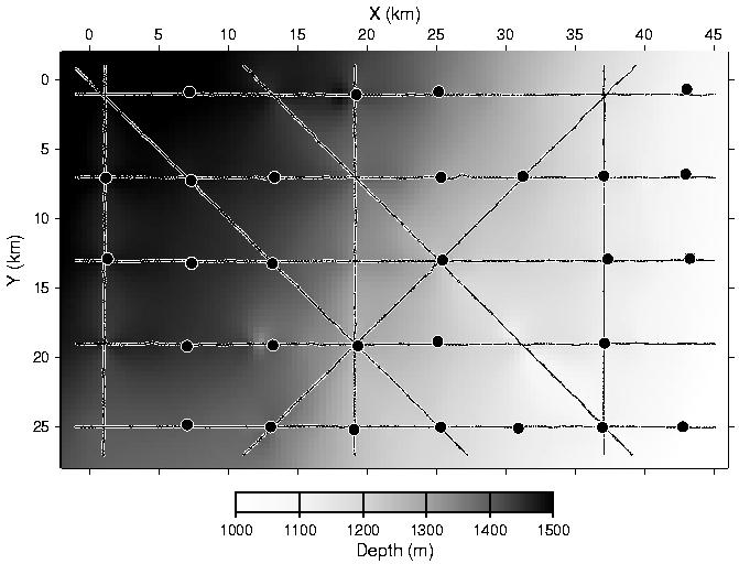
Figure 1. 3D Faeroe Basin experiment geometry and bathymetry. Large dots show the 29 OBS locations and small dots along the 11 profiles show the 3800 airgun shot points.
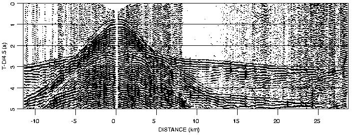
Figure 2. Example of the Faeroe Basin refraction data plotted using reduced traveltime (4.5 km/s) versus source-receiver offset. A 1-12 Hz bandpass filter has been applied. The data quality of this record section is average for the data set as a whole.
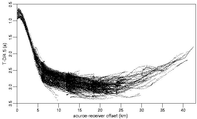
Figure 3. Complete set of 53,479 picks reduced at 4.5 km/s and plotted versus source-receiver offset without regard to position or azimuth. Solid line represents the average time in 1 km offset bins.
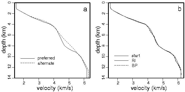
Figure 4. (a) Preferred and alternate 1D starting velocity models. (b) Comparison of preferred starting model and 1D average of final models obtained using regularized inversion (RI) and backprojection (BP).
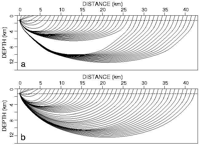
Figure 5. Raypaths through (a) preferred and (b) alternate starting model. Dashed line represents average position of water-sediment interface in study area.
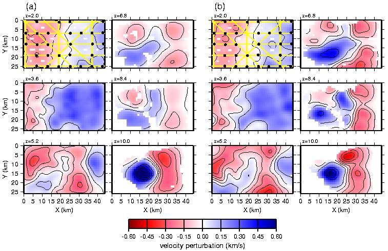
Figure 6. Preferred final models from (a) regularized inversion and (b) backprojection using the preferred starting model. See text for details of how each model was obtained. Perturbations with respect to the starting model are shown for depths from z=2 km to z=10 km as labeled. For reference, OBSs and shot lines are shown over the z=2 km plots. Regions not sampled by raypaths are blank. Contour interval is 0.1 km/s.
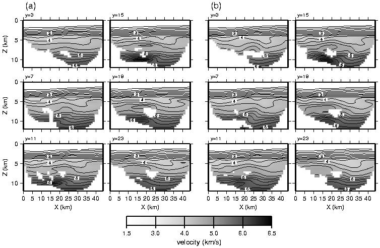
Figure 7. Preferred final models from (a) regularized inversion and (b) backprojection using the preferred starting model. See text for details of how each model was obtained. Velocity shown at vertical positions from y=3 km to y=23 km as labeled. Regions not sampled by raypaths are blank. Contour interval is 0.25 km/s.
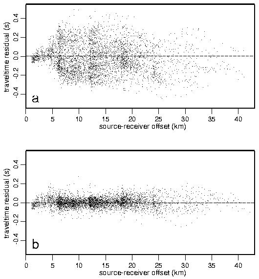
Figure 8. Traveltime residuals as a function of offset for (a) preferred starting model and (b) preferred final model from regularized inversion. For clarity, only every tenth residual is plotted. All inversions of the real data presented in this paper provide a similar traveltime residual plot.
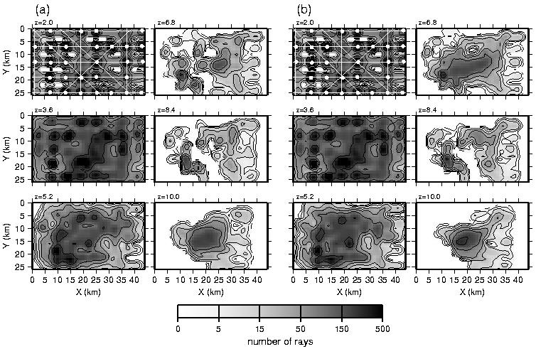
Figure 9. Ray coverage in the preferred final model from (a) regularized inversion and (b) backprojection using a 1.2´1.2´0.4 km cell size. For reference, OBSs and shot lines are shown over the z=2 km plots. Regions not sampled by raypaths are blank. Contour values are 0, 2, 5, 10, 25, 50, 100, 250, and 500.
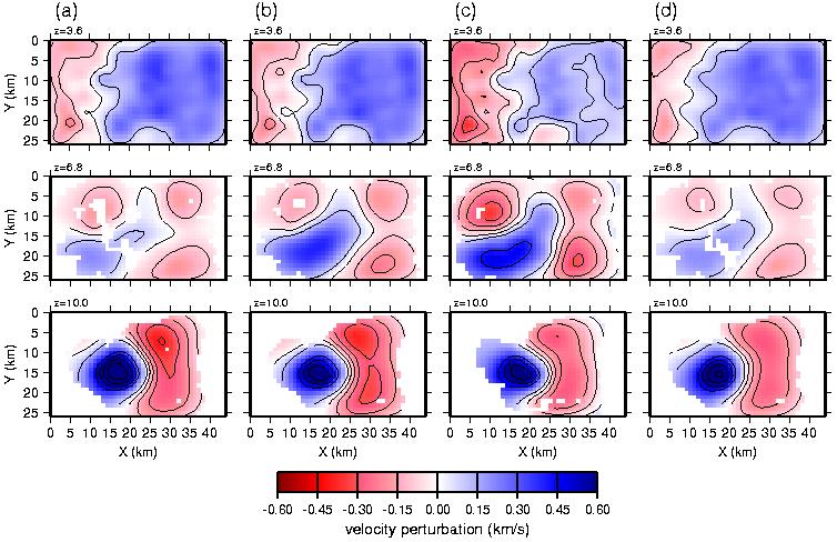
Figure 10. Final models from regularized inversion. (a) Using a vertical/horizontal smoothness constraint (sz) of 0.075. (b) Using a vertical/horizontal smoothness constraint (sz) of 0.25. (c) Using the alternate starting model. (d) Inversion of synthetic data calculated from the preferred final model (Figures 6a). Regions not sampled by raypaths are blank. Contour interval is 0.1 km/s.
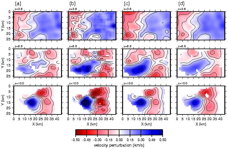
Figure 11. Final models from backprojection. (a) Using a constant horizontal´vertical MA operator size of 4.4´1.2 km for the smoothing schedule. (b) Using the Hole [1992] backprojection method. (c) Using the alternate starting model. (d) Inversion of synthetic data calculated from the preferred final model (Figures 6b). Regions not sampled by raypaths are blank. Contour interval is 0.1 km/s.
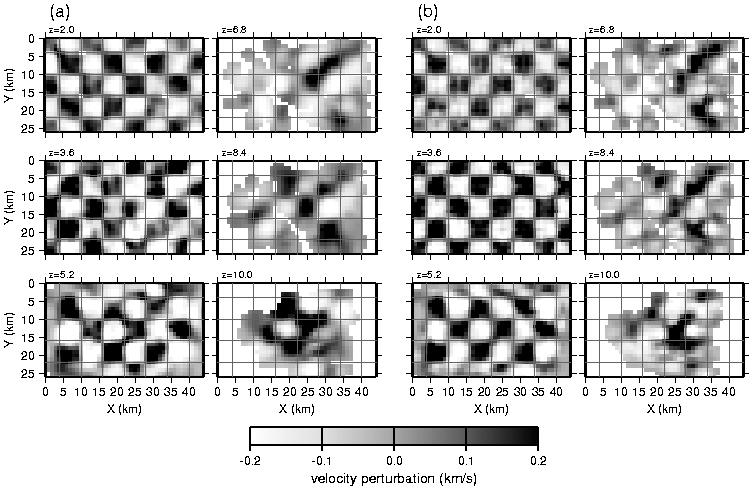
Figure 12. Results of checkerboard test for (a) regularized inversion and (b) backprojection. Velocity perturbations with respect to starting model are shown for depths from z=2 km to z=10 km as labeled. True checkerboard pattern is ±0.2 km/s in 6x6 km squares as indicated by the grid lines. Regions not sampled by raypaths are blank.
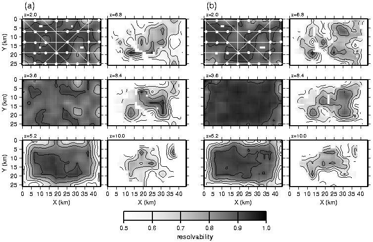
Figure 13. Resolvability of final model from (a) regularized inversion and (b) backprojection. Resolvability at each point equals the semblance between the exact and recovered checkerboard models (Figure 12) using a 6x6x1.2 km operator. For reference, the OBSs and shot lines are shown over the z=2 km plots. Regions not sampled by raypaths are blank. Contour interval is 0.1.
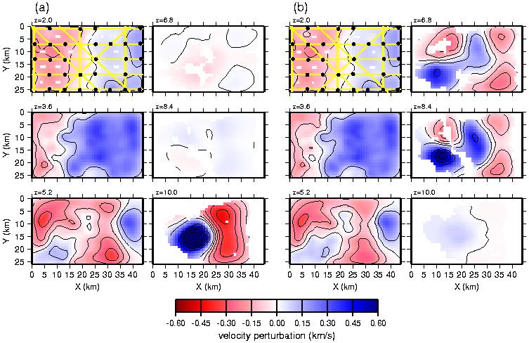
Figure 14. Final models from regularized inversion using a strong flatness constraint between (a) z=6.6 km and z=8.6 km to assess the poorly constrained depth range of the model, and (b) z=9 km and z=14 km to assess the depth range which contains the largest velocity anomaly (Figure 6). For reference, OBSs and shot lines are shown over the z=2 km plots. Regions not sampled by raypaths are blank. Contour interval is 0.1 km/s.
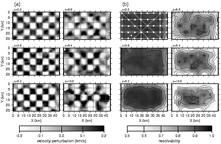
Figure 15. (a) Results of checkerboard test for regularized inversion assuming there was 100% recovery of data from all 40 OBSs deployed. Velocity perturbations with respect to starting model are shown for depths from z=2 km to z=10 km as labeled. True checkerboard pattern is ±0.2 km/s in 6x6 km squares as indicated by the grid lines. (b) Corresponding resolvability of final model. Resolvability at each point equals the semblance between the exact and recovered checkerboard models using a 6x6x1.2 km operator. For reference, the 40 OBSs and shot lines are shown over the z=2 km plot. Contour interval is 0.1. Regions not sampled by raypaths are blank.
Figure 16. Maximum difference between final models from regularized inversion and backprojection using a range of free parameters for each method corresponding to the models shown in Figures 6, 10a, 10b, and 11a. For reference, OBSs and shot lines are shown over the z=2 km plots. Regions not sampled by raypaths are blank. Contour interval is 0.1 km/s.