Strategies for modelling seismic refraction/wide-angle reflection traveltimes to obtain 2-D velocity and interface structure are presented along with methods for assessing the reliability of the results. Emphasis is placed on using inverse methods, but a discussion of arrival picking and classification, data uncertainties, traveltime reciprocity, crooked line geometry, and the selection of a starting model is also applicable to trial-and-error forward modelling. The most important advantages of an inverse method are the ability to derive simpler models for the appropriate level of fit to the data, and the ability to assess the final model in terms of resolution, parameter bounds and non-uniqueness. Given the unique characteristics of each dataset and the local earth structure, there is no single approach to modelling wide-angle data that is best. This paper describes the best modelling strategies according to the (1) model parameterization, (2) inclusion of prior information, (3) complexity of the earth structure, (4) characteristics of the data, and (5) utilisation of coincident seismic reflection data. There are two natural end member inversion styles: (1) a regular, fine-grid parameterization when seeking a minimum-structure model, and (2) an irregular grid, minimum-parameter model when considering certain forms of prior information. The former style represents the "pure" tomography approach. The latter style is closer to automated forward modelling, and can be applied best with a parameter-selective algorithm, that is, one that allows any subset of model parameters to be selected for inversion. If there is strong lateral heterogeneity in the near-surface only, layer stripping works well. If there is complexity at all depths, all model parameters should be determined simultaneously after careful construction of a starting model that allows the appropriate rays to be traced to all pick locations. The lateral spacing of model nodes to use will depend on the type of inversion and whether detailed prior information is included, but a general guideline based on model resolution when seeking a minimum-parameter model is a model node spacing equal to the shot spacing (receiver spacing for typical marine data), except perhaps in the upper layers where about half this may be necessary; node spacing is not an issue when using smoothing constraints provided it is small enough to resolve the earth structure of interest. Traveltimes picked from pre-stack, unmigrated or migrated coincident reflection data can be (1) used to develop the starting model, (2) inverted simultaneously with the wide-angle data, or (3) inverted after modelling the wide-angle data to constrain interfaces that "float" within the velocity model. Model assessment establishes the reliability of the final model. Presenting model statistics, traveltime fits, ray diagrams, and resolution kernels is useful, but can only indirectly address this issue. Direct model assessment techniques that derive alternative models that satisfactorily fit the real data are the best means for establishing the absolute bounds on model parameters and whether a particular model feature is required by the data.
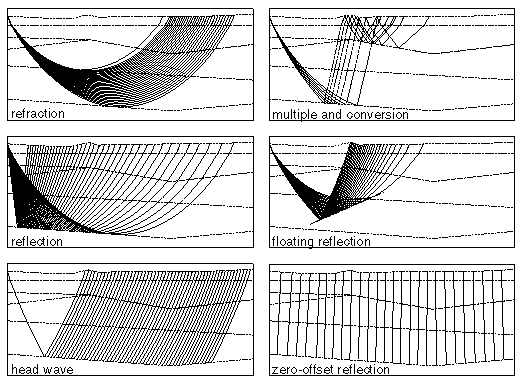
Examples of the types of ray groups considered for wide-angle traveltime modelling. Solid lines are raypaths and dashed lines are layer boundaries. Dotted lines indicate S-wave segments for converted raypaths. A "floating" reflection arises from an interface, indicated by a dotted line, that is not associated with a velocity discontinuity.
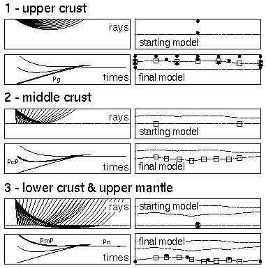
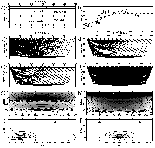
Example of the "across-and-down" modelling approach (Zelt & Smith 1992). The upper crust, middle crust and lower crust/upper mantle are determined in three layer-stripping steps, using the appropriate phases at each step to progressively develop the model by adding nodes across the model in each layer to define the structure needed to satisfactorily fit the observed traveltimes before proceeding to deeper layers. For each step, an example of the rays for one shot is shown above the corresponding traveltime curves for all phases with the phases of interest labelled and indicated by a thicker line. The phases are Pg - upper crustal refraction, PcP - mid- crustal reflection, PmP - Moho reflection, and Pn - upper mantle refraction. The two models shown to the right for each step represent the starting model (above) and final model (below) in each case. Circles and open squares indicate velocity and depth nodes, respectively. Note that the layers being solved for start out laterally homogeneous in each step.
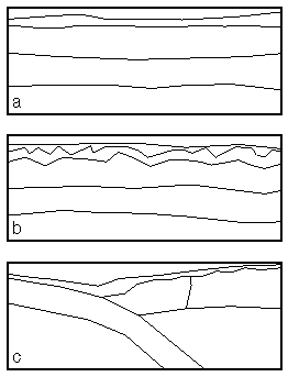
Structural classification of model types. (a) Weak lateral heterogeneity at all depths. (b) Strong lateral heterogeneity in the upper part of the model, but weak lateral heterogeneity below. (c) Strong lateral heterogeneity at all depths. Based on crustal-scale examples of cratonic crust, extended crust, and a convergent margin.
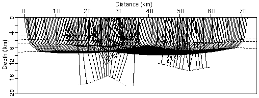
Example of joint wide-angle and zero-offset traveltime inversion with floating reflectors from a marine survey on the Iberia margin (Sawyer et al. 1998). Zero-offset reflections from the second and fourth layer boundaries that were picked from unmigrated reflection data have been inverted simultaneously with first arrival refractions to constrain the 2-D velocity and interface structure. Subsequently, other zero-offset reflections were modelled using floating reflections located mainly in the fifth model layer. Raypaths are thick for zero-offset reflections and thin for refractions; layer boundaries are long dashed lines; floating reflectors are short dashed line segments.
Examples of plots used for indirect model assessment. (a) Four layer crustal model. Layer boundaries are dashed lines; velocity and depth nodes indicated by circles and squares. (b) Traveltime data reduced using 8 km/s for a shot at 0 km. The phases are Ps - sediment refraction, Pg - upper crustal refraction, PcP - mid-crustal reflection, Pc - lower crustal refraction, PmP - Moho reflection, and Pn - upper mantle refraction. (c) Non-two-point ray diagram for a shot a 0 km and the phases shown in (b). (d) Two-point ray diagram for a shot a 0 km. (e) Two-point ray diagram for a shot at 0 km including only the first-arriving raypath for each phase. (f) Same as (e) but for 11 shots intended to represent the complete dataset. (g) Ray hit counts for the raypaths in (f) displayed in contour format and shading for velocity nodes (darkness of grey increases with hit counts) and symbol size for depth nodes (circle size increases with hit counts). (h) Diagonal values of resolution matrix for the raypaths in (f) displayed in contour format and shading for velocity nodes (darkness of grey increases with diagonal value) and symbol size for depth nodes (circle size increases with diagonal value). (i) Resolution kernel for a velocity node at the base of the crust at x=50 km and the raypaths in (f) displayed in contour format and shading for velocity nodes (darkness of grey increases with resolution kernel value) and symbol size for depth nodes (circle size increases with resolution kernel value). (j) Same as (i) but for a node at x=150 km. For clarity, every third traveltime and raypath are shown.
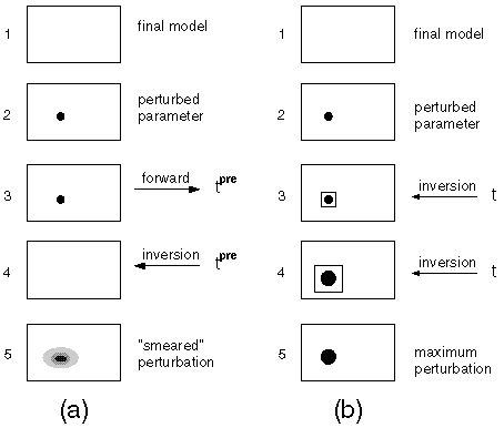
Single-parameter resolution and uncertainty tests. The five main steps of each test are shown in schematic form, starting with (1) a final model, and (2) the selection and perturbation of one model parameter indicated by the black dot. (a) To estimate the spatial resolution centred about the chosen parameter, the remaining steps are (3) calculation of the perturbed dataset, tpre, (4) inversion of the perturbed data set using the final model as a starting model, and (5) examination of the recovered and typically smeared perturbation. (b) To estimate the absolute uncertainty of the chosen parameter, the remaining steps are (3) inversion of the real dataset, t, fixing the value of the perturbed parameter, indicated by the square surrounding the perturbed parameter, (4) increasing the size of the perturbation until the largest perturbation is determined that will allow a satisfactory fit of the real data, and (5) the maximum allowable perturbation is the absolute parameter uncertainty.
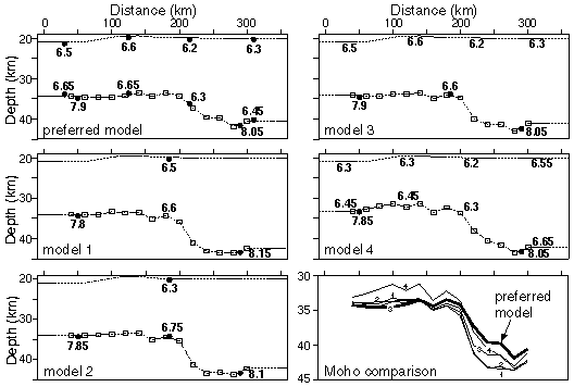
Example of multi-parameter model assessment from Zelt & White (1995). The preferred final model is compared with four alternate models of lower crustal-upper mantle structure. Dashed lines are layer boundaries and velocity in km/s is indicated for each node. Traveltime inversion of PmP and Pn was used to determine the lower crustal velocities indicated by black dots (other lower crustal velocities not associated with black dots were held fixed), as well as the Moho (depth nodes indicated by squares) and upper mantle velocities. The lower right diagram is a close-up comparison of the five Mohos.