Colin. A. Zelt
Department of Geology and Geophysics, Rice University
6100 Main Street, Houston, Texas, 77005-1892, USA
Barry. C. Zelt
Geotechnology Research Institute, Houston Advanced Research Center
4800 Research Forest Drive, The Woodlands, Texas, 77381, USA
(now at:
Department of Earth and Ocean Sciences, University of British Columbia
2219 Main Mall, Vancouver, British Columbia, V6T 1Z4, Canada)
Tectonophysics, 286, 209-221, 1998.
In the presence of three-dimensional (3D) inhomogeneous structure, the results of 2D traveltime inversion will be in error since the effects of "out-of-plane" or 3D ray sampling are ignored. We have inverted synthetic data using 2D and 3D algorithms to examine the errors caused by 3D inhomogeneities which produce significant out-of-plane ray bending. The results of inverting data from 2D experiments are compared with vertical slices through 3D models obtained by inverting data using a number of recently-employed 3D recording geometries. Our results show that, even for strong 3D inhomogeneities, out-of-plane effects are relatively small, with crustal velocity errors of less than 0.15 km/s, and intra-crustal boundary depth errors generally less than 2 km. These errors are approximately equal to the uncertainties commonly assigned to crustal models derived from traveltime inversion. The artifacts are also similar in magnitude to the lateral smearing that occurs in 3D models when using relatively coarse 3D geometries. Only for a dense network of profiles will a 3D inversion using off- and in-line data provide greater lateral resolution than a 2D independent or simultaneous inversion of in-line data along each profile. 2D and 2.5D inversion of crooked-line data in the presence of strong velocity variations produces erroneous small-scale velocity structure. We conclude that most 3D crustal experiments cannot be justified on the basis that the results from a 2D experiment or a network of 2D profiles will be significantly in error due to out-of-plane effects. 3D experiments can be justified when a dense grid of shots and receivers is used or if a volume image, as opposed to a cross-sectional image, is required.

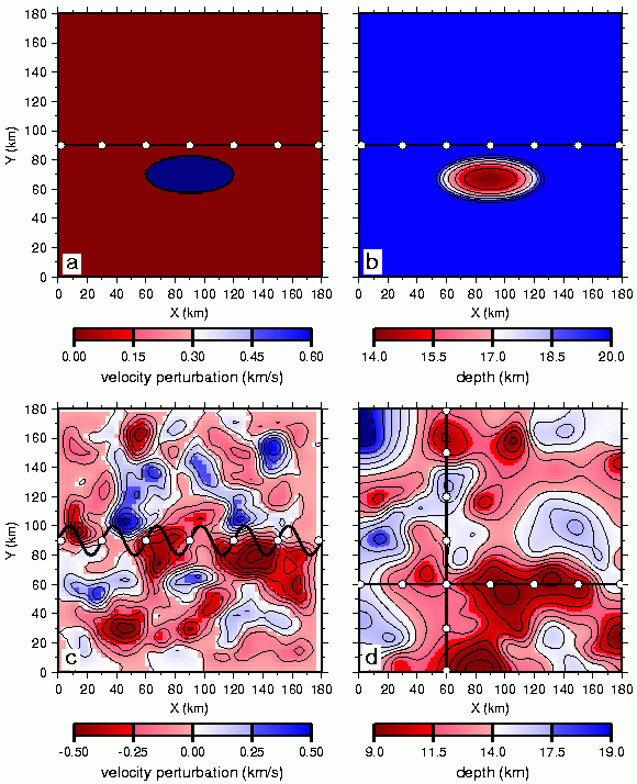
Fig. 1. True models. (a) Single-perturbation velocity model with an anomaly of +10% with respect to the background model between 4-7 km depth. (b) Single-perturbation reflector model with an anomaly having a peak amplitude of 6 km with respect to the background model depth of 20 km. (c) Random velocity model with variations up to 10% (0.6 km/s) with respect to the laterally homogeneous background model; horizontal slice at z=1 km is shown and is typical of entire model. (d) Random reflector model with an average depth of 13 km and maximum variations of 6 km. The background velocity model has been subtracted for the plots in (a) and (c). The straight-line 2D geometry is superimposed on the single-perturbation models in (a) and (b), the crooked-line geometry is superimposed on the random velocity model in (c), and the two profiles used for 2D experiments are superimposed on the random reflector model in (d). Shot points indicated by white dots and receivers spaced at 1 km are located along each line. Contour interval is 0.1 km/s in (c) and 1 km in (b) and (d).
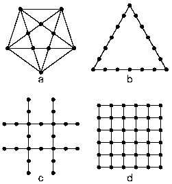
Fig. 2. 3D geometries. Shot points are indicated by dots; receivers spaced at 1 km are located along the lines. (a) star, (b) triangle, (c) coarse-grid, and (d) fine-grid geometry.
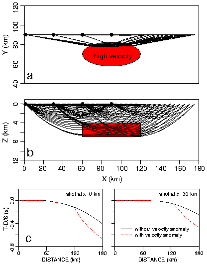
Fig. 3. Ray tracing for the 2D experiment using the true single-perturbation velocity model (Fig. 1a). (a) Plan view shows rays bending out of plane through high-velocity anomaly (red ellipse). (b) Side view shows ray coverage projected into x-z plane; the red rectangle between 4-7 km depth outlines the velocity anomaly. Dots are shot points. Because of symmetry, rays from the three right-most shots are equivalent to those from the three left-most shots and are omitted for clarity. (c) Calculated traveltimes for the shots at x=0 km and x=30 km for the background model (solid line) and with the velocity perturbation (dashed line); times reduced using 6 km/s.
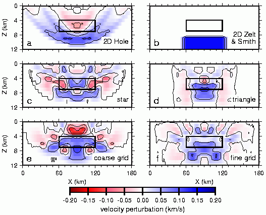
Fig. 4. Results of velocity inversion for the single-perturbation model (Fig. 1a). 2D experiment using (a) Hole (1992) method and (b) Zelt and Smith (1992) method, and slices at y=90 km through recovered models from using (c) star, (d) triangle, (e) coarse-grid, and (f) fine-grid 3D geometry. In all cases, the anomaly has been imaged at a greater depth and with a lower magnitude than the true anomaly. Rectangle indicates the out-of-plane position of the true ellipsoidal velocity anomaly (Fig. 3). Contour interval is 0.1 km/s.
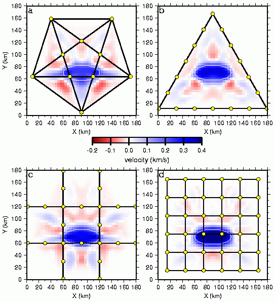
Fig. 5. Results of 3D velocity inversion for single-perturbation model (Fig. 1a) using (a) star, (b) triangle, (c) coarse-grid, and (d) fine-grid 3D geometry. Horizontal slices through the 3D models represent the average of the recovered models minus the laterally homogeneous background model averaged over the depth range (4-7 km) spanned by the true velocity anomaly. White ellipse indicates position of true velocity anomaly. Dots represent shot point locations; straight lines denote receiver profiles. Contour interval is 0.1 km/s.
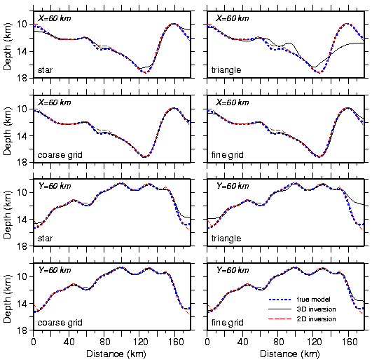
Fig. 6. Comparison of 2D and 3D inversions at x=60 km and y=60 km for the random reflector model (Fig. 1d). Thick, short dashed line represents depth to the true reflector. Thin, solid line represents depth to the recovered reflector in the 3D models for the 3D geometries as labeled. Thin, long dashed line represents depth to the reflector from the 2D inversions.
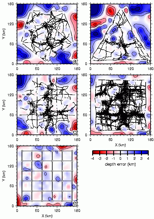
Fig. 7. Results of 3D depth inversion for the random reflector model (Fig. 1d). The difference between the true and recovered reflector depths is shown for the (a) star, (b) triangle, (c) coarse- grid, and (d) fine-grid 3D geometry. The PcP reflection points associated with each final model are superimposed on each plot. (e) Results of simultaneous 2D network inversion for the random reflector model showing the difference between the true reflector model and that obtained by contouring the depth estimates available along each of the 12 straight profiles comprising the network; dots represent shot point locations; straight lines denote receiver profiles. Contour interval is 1 km.
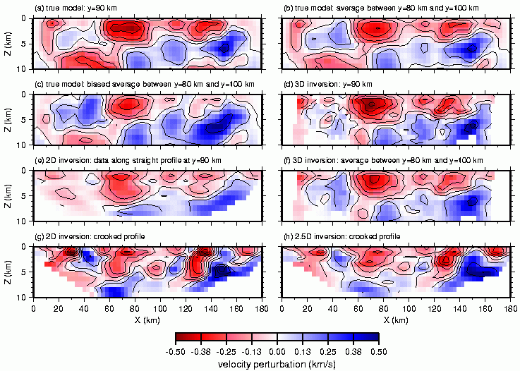
Fig. 8. Results of inverting crooked-line data using the random velocity model (Fig. 1c). Perturbations from the linear gradient background model are shown for the models as labeled above each figure. Regions of no ray coverage have been omitted. Contour interval is 0.1 km/s.